How to speed up python code for Machine Learning: The ALeRCE light curve classifier experience
The ALeRCE light curve classifier
The Automatic Learning for the Rapid Classification of Events (ALeRCE) alert broker1 is a service that connects to different telescopes around the world, receives astronomical alerts, and does processing and analysis over them in order to provide useful information to the astronomical community. One of the tasks that ALeRCE does is to classify hundreds of thousands of objects in different astrophysical categories, like supernova, cepheid stars, active galactic nuclei, to name a few classes. The results of the classifier are publically available to anyone through a webpage, an API and a database, so they can be used by astronomers to do further scientific research.
One of the classifiers that is running on ALeRCE is the light curve classifier2, a model that takes the light curve of an object, computes features, applies a random-forest based classifier and returns a vector of probabilities. A light curve is a time series that represents the evolution of the brightness of an object through time. For example this figure shows the light curve of a type II supernovae obtained by the Zwicky Transient Facility (ZTF).
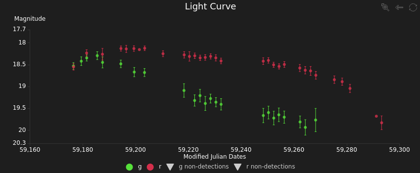
You can see more information about this object in the ALeRCE explorer.
Considering that ALeRCE is receiving hundreds of thousands of alerts every night, it’s crucial for the operation of our data pipeline to perform the classifications as fast as possible. Nonetheless, almost all of the implementation of the light curve classifier is done using python (and is available in github), which is not precisely known for being fast.
In this post I will present some of the things that we have learnt during the development and operation of the light curve classifier, in particular, how we have improved its speed.
General advices
1. “A good design is far more important than optimization.”
Think first on the structure of your code and make sure it is easy to extend and non redundant. Put your effort on writing clear, easy-to-understand code. Be kind with the other programmers and with your future self.
Why? Because software engineering hours are very expensive.
2. Do profiling
If you care about performance you have to measure the time. Don’t guess what function is slowing down your code because you will probably be wrong. It’s very common to discover that some random function is in fact the slowest one, maybe because of a couple of very inefficient lines of code or a call to an API in another server, etc.
Please, do profiling. Don’t spend hours of days optimizing the wrong thing. Remember, software engineering hours are very expensive.
3. Do the work once
Are you computing the same thing many times? If you are performing the same operation many times you could calculate once, save the result and re-use in the future. This is a basic idea in computer science (e.g. memoization) and can save your life.
Python provides a native implementation through decorators. Just import lru_cache and decorate your function as follows:
from functools import lru_cache

@lru_cache(64)
def factorial(n):
    ans = 1.0
    for i in range(n+1):
        ans *= i
    return ans
By including this decorator, python will remember the answer to your function and it will not compute it again if it’s not necessary. The value 64 in the decorator means that only the last 64 calls with different arguments will be kept in memory.
This will only be useful if the same computation repeats in the future, not if it is changing every single time. Another detail is that you are trading off computation time for memory, which is also a limited resource.
4. Parallelize in the right place
One common way to speed up a program is to parallelize its execution and running it in many cores or multiple machines. One key decision is to break the problem in the right place. In our case we have to classify multiple objects, compute many features for each of them and many features could be broken into pieces of code that run in parallel (e.g. break up a multiplication of two matrices).
Let’s compare these cases. A matrix multiplication could be broken up into the multiplication of smaller matrices, but at the end the results of those operations have to be joined together to get the final result. It might be even necessary to do some extra calculations over the partial results before computing the final results, and the final result will only be available after the slowest of the partial computations is done.
In contrast, each light curve is independent from each other, so splitting up the problem here is trivial. You only need to run many instances of the classifier and feed them with different light curves. This kind of situation is said to be embarrassingly parallel, so this was the natural choice in ALeRCE.
Python profiling
To profile our code we used cProfile, the recommended python profiler. It will record every function call and how much time did it take. It’s not the only kind of profiling that exists (line profilers, stochastic profilers) but it’s super useful and powerful.
I have used this profiler in two ways. The easiest one is to call it from a terminal and profile the execution of a whole python script:
>> python -m cProfile -o profiling_output.prof my_script.pyThat will run my_script.py and save the result of the profiling in profiling_output.prof. The second way is to modify your code and use a Profiler object.
import cProfile
profiler = cProfile.Profile()
profiler.enable()

# your code goes here

profiler.disable()
profiler.dump_stats("profiling_output.prof")
The advantage of the second way is that you have more control over what part of the code you are measuring. For example, you might want to avoid measuring times when importing libraries or creating objects and just focus on the lines where the classification is done.
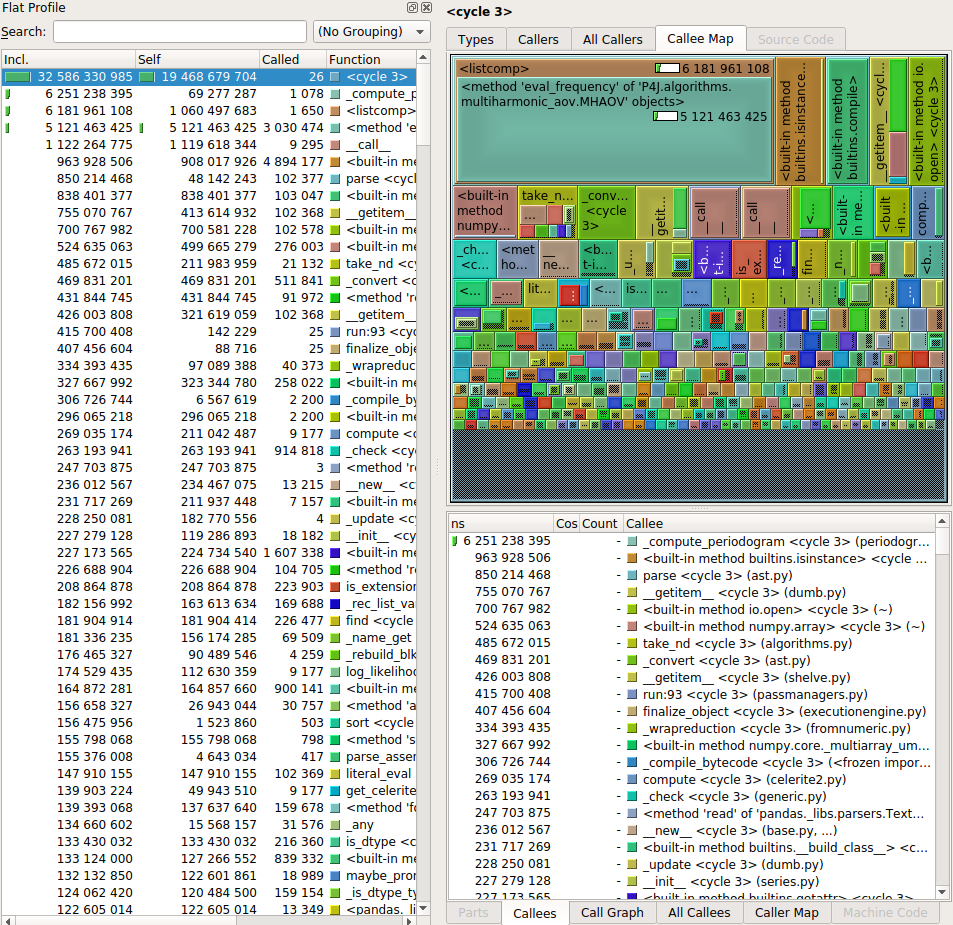
After that you will need a way to visualize the output of the profiling. I have used two tools: snakeviz and kcachegrind. Both offer similar tools like a visualization and a table with the called functions, indicating the time spent on each call, the number of calls, etc. Let’s see a couple of screenshots.
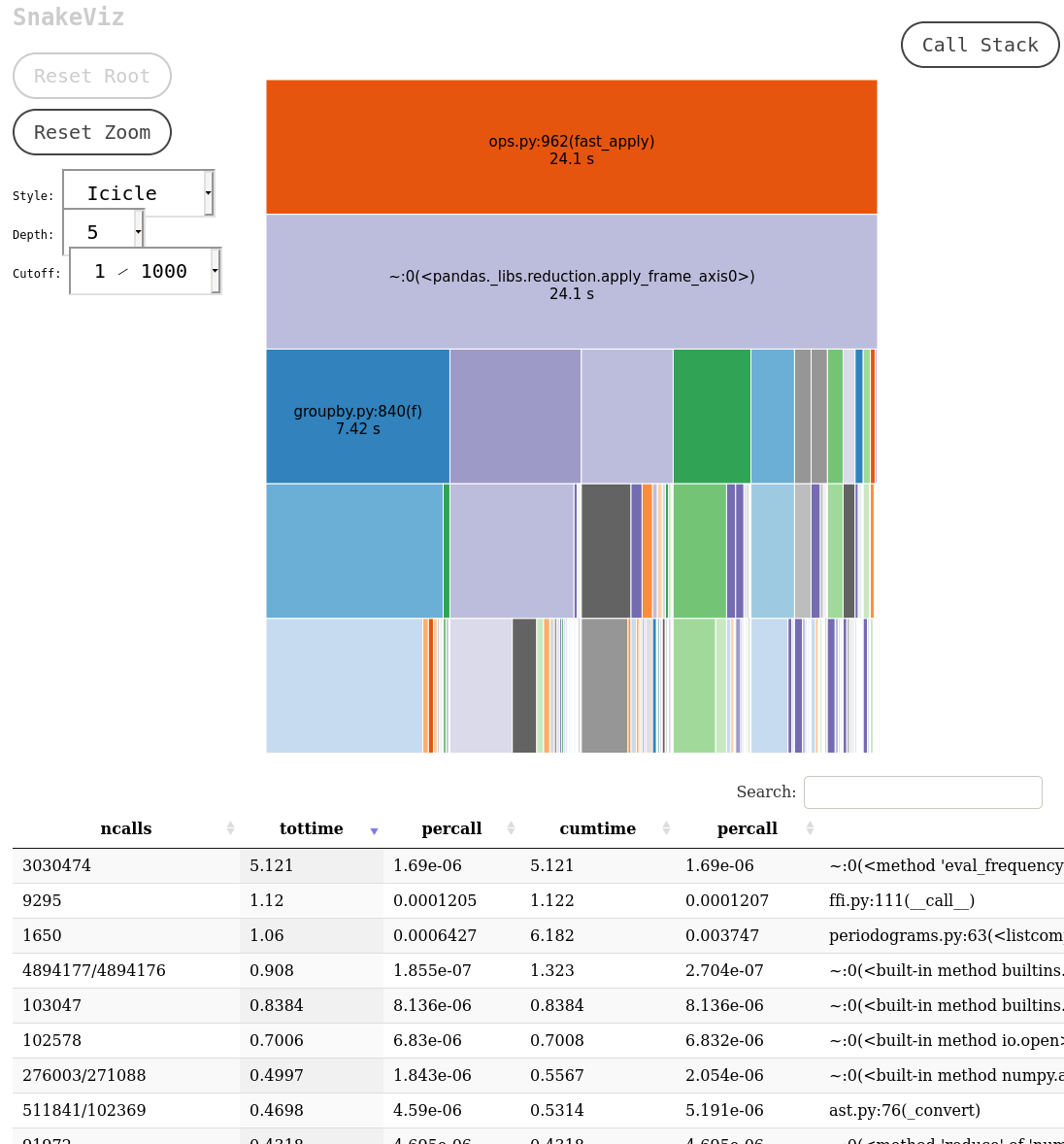
These programs make it very easy to identify the most critical pieces of code, which allows the programmer to spend its time optimizing the code that will make a difference. A couple of things to look in detail are the functions with the largest self-time, the functions that are called many times and the functions that take a long time per call.
One of the pitfalls that I found while doing the profiling has to do with inheritance and polymorphism. In our code we have many feature extractors, each one responsible for computing a statistic from the light curve, and they are implemented as classes that inherit from a base class. In consequence, our code has many implementations of the abstract method “compute_feature”, which makes the profiler visualizer a little bit “dizzy”. Using both snakeviz and kcachegrind makes it easier to remedy this situation and understand what is happening with your code.
Using numba
Numba is a python package that allows you to speed up functions by just adding a decorator. Numba performs a just-in-time compilation under the hood, which can let python reach the performance of low level compiled languages. Your function is restricted to contain native python code plus numpy, but that is a very powerful combination if you are doing scientific computing. Another limitation (that might change in the future) is that you can only accelerate functions, not methods from a class.
In ALeRCE we are using numba in the computation of many features like the conditional autoregressive model, the structure function, the irregular autoregressive model and the supernova parametric model. Those functions were taking a relevant fraction of time according to the profiling, and when inspected we noticed that they were not using any external package besides numpy, making them excellent candidates for numba.
As an example of how to use numba, this is a function used by our supernova parametric model:
from numba import jit
import numpy as np

@jit(nopython=True)
def model_inference(times, A, t0, gamma, f, t_rise, t_fall):
    beta = 1.0 / 3.0
    t1 = t0 + gamma

    sigmoid = 1.0 / (1.0 + np.exp(-beta * (times - t1)))
    den = 1 + np.exp(-(times - t0) / t_rise)
    flux = (A * (1 - f) * np.exp(-(times - t1) / t_fall) / den
         * sigmoid
         + A * (1. - f * (times - t0) / gamma) / den
         * (1 - sigmoid))
    return flux
The model_inference function has only python and numpy instructions, making it ideal for optimization with numba. Make sure that you are using “nopython=True”, which means that your code will fail if the compilation of your function has a problem. Otherwise, if there is a problem during compilation numba will fall back to the python plus numba function that you wrote.
The process is not always straightforward. One of the restrictions is that you don’t change the shape and dtype of your numpy variables. My advice is to add the decorator @jit(nopython=True), use the function and debug if it fails. What you have to look at are the types of your variables, and for the case of numpy arrays check their shapes and dtypes.
Using Cython
Cython is another way to get the performance of a low level language using python by just adding some annotations to your python code. The idea is to include some extra information like types in your python code, and then Cython is capable of building an equivalent code in C that can be called from python.
Cython is an extension of the python language designed to be easily transformed into C. In consequence, having previous experience with C can be very useful to deal with the learning curve of Cython, which is quite steeper compared to numba.
In ALeRCE we have used Cython in two pieces of code. The first one is the library P4J for estimating periods of light curves, developed by Pablo Huijse. Period computation is probably the most expensive operation in the ALeRCE pipeline, so having a fast implementation is key.
The other use of Cython in ALeRCE is the Mexican Hat Power Spectra (MHPS), based on the work of Patricia Arévalo. This is used as a feature in the light curve classifier. As the original code was written in C, choosing Cython was a natural choice to include MHPS in our pipeline and keep the low level performance.
Beside the performance tips that you can find in Cython’s documentation, we have found a couple of details that you might want to keep an eye on. As Cython translates your “extended python” code into C, that means that when you install your package that C code has to be compiled. Although it might look like an overkill, disassembling the binary and reading the assembly instructions generated by the compiler can be useful.
In our case the first thing we noticed was that the compiled library was not using all the instruction sets available in the machine, like AVX2 or AVX512. This is the default behaviour of the compiler, but it reminded us to give the compiler the right flags to take advantage of the hardware. These flags are -O3 (for heavy optimization), -ffast-math and -march=native. The ffast-math flag allows the compiler to ignore some strict rules about math operations (like associativity), but you should check your compiler documentation to be sure that you don’t rely on any of those rules. The flag march=native tells the compiler that it can use all the available instruction sets in your machine.
Another thing that we noticed while reading the disassembled binary was some conversions between single precision floats and double precision floats, despite we were using only single precision variables in our code. Of course we were not, and there were some hidden doubles that we missed. Let’s see an example:
arg = 2.0 * M_PI * (arg - floorf(arg))The variables arg and M_PI were declared as floats, and the function floorf returns a float. The problem is that Cython is an extension of python, and 2.0 is a double precision float in python. What the code was doing in reality was the following:
arg = (float) ((2.0 * (double)M_PI) * (double)(arg - floorf(arg)))That means that in that line were hidden casting operations, two float to double castings and a double to float casting. Of course this is not an important performance loss, but now that we know that is there we can easily fix it with this trick:
cdef float two_float = 2.0
arg = two_float*M_PI*(arg - floorf(arg))-
Förster, F., et al. “The Automatic Learning for the Rapid Classification of Events (ALeRCE) Alert Broker.” arXiv preprint https://arxiv.org/abs/2008.03303 (2020). ↩
-
Sánchez-Sáez, P., et al. “Alert classification for the alerce broker system: The light curve classifier.” The Astronomical Journal 161.3 (2021): 141. Link to pdf ↩